Structural Equation Modelling

fit.1 <- lm(wage ~ age, data = Wage)

Structural Equation Models (SEM) help to model the dependence relationships among multiple variables, simultaneously. In other words, we can model not only multiple variables, but each of those dependent variables can have multiple covariates attached to them.

Software

There are a plethora of options available to create SEMs. Here are just a few of them:

1. lavaan
2. MPlus
3. SAS
4. Stata

This project will use the lavaan library. If you don't have it installed, simply run the following command in your IDE of choice:

# install.packages("lavaan", dependencies=TRUE)
library(lavaan)

BTW, this walk-through is my interpretation of the fantastic guide created by UCLA.

Introduction

Structural equation modeling is a linear model framework that models concrete regression equations with latent variables.

Motivating Example

Suppose you are a researcher studying the effects of student background on academic achievement. The lab recently finished collecting and uploading the dataset (worland5.csv) of $N= 500$ students with $9$ observed variables for each student. The principal investigator hypothesizes three latent constructs Adjustment, Risk, Achievement measured with its corresponding to the following codebook mapping:

Adjustment:

• motiv - Motivation

• harm - Harmony

• stabi - Stability

Risk:

• ppsych - (Negative) Parental Psychology

• ses - Socio-economic Status

• verbal - Verbal IQ

Achievement:

• read - Reading

• arith - Arithmetic

• spell - Spelling

Here's how to download and load the dataset into R:

dat <- read.csv("https://stats.idre.ucla.edu/wp-content/uploads/2021/02/worland5.csv")

Key

The most essential component of a structural equation model is covariance or the statistical relationship between items. The true population covariance, denoted $\Sigma$, is called the variance-covariance matrix. Since you don't ever know the true $\Sigma$, you can estimate it with your sample data. We call this the sample variance-covariance matrix, or $\hat{\sigma}$.

The variance-covariance matrix $\Sigma$ should not be confused with $\Sigma(\theta)$ which is the model. However, if the model fits perfectly, then $\Sigma = \Sigma(\theta)$.

Running the cov command in R allows us to obtain the population variance-covariance matrix $\Sigma$?

Answer: False, the cov command obtains the sample, or $S$.

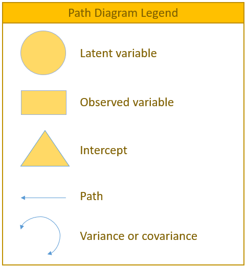
Definitions

• observed variable: a variable that exists in the data, a.k.a item or manifest variable

• latent variable: a variable that is constructed and does not exist in the data

• exogenous variable: an independent variable either observed (x) or latent ($\Xi$) that explains an endogenous variable

• endogenous variable: a dependent variable, either observed (y) or latent ($\eta$) that has a causal path leading to it

• measurement model: a model that links observed variables with latent variables

• indicator: an observed variable in a measurement model (can be exogenous or endogenous)

• factor: a latent variable defined by its indicators (can be exogenous or endogenous)

• loading: a path between an indicator and a factor

• structural model: a model that specifies causal relationships among exogenous variables to endogenous variables (can be observed or latent)

• regression path: a path between exogenous and endogenous variables (can be observed or latent)

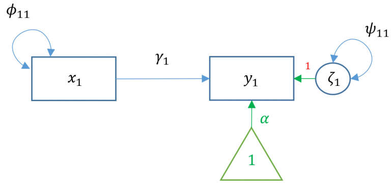
• $x_1$, a single exogenous variable

• $y_1$, single endogenous variable

• $\beta_0, \alpha_1$, intercept of $y_1$, "alpha"

• $\beta_1, \gamma_1$, regression coefficient, "gamma"

• $\phi$, variance or covariance of the exogenous variable, "phi"

• $\psi$, residual variance or covariance of the endogenous variable, "psi"

The path model

lavaan syntax

Before running our first regression analysis, let us introduce some of the most frequently used syntax in lavaan

• ~ predict, used for regression of observed outcome to observed predictors (e.g., y ~ x)

• =~ indicator, used for latent variable to observed indicator in factor analysis measurement models (e.g., f =~ q + r + s)

• ~~ covariance (e.g., x ~~ x)

• ~1 intercept or mean (e.g., x ~ 1 estimates the mean of variable x)

• 1* fixes parameter or loading to one (e.g., f =~ 1*q)

• NA* frees parameter or loading (useful to override default marker method, (e.g., f =~ NA*q)

• a* labels the parameter 'a', used for model constraints (e.g., f =~ a*q)

Simple regression

Simple regression models the relationship of an observed exogenous variable on a single observed endogenous variable. For a single subject, the simple linear regression equation is most commonly defined as:

In R, the most basic way to run a linear regression is to use the lm() function:

#simple regression using lm()
m1a <- lm(read ~ motiv, data=dat)
(fit1a <-summary(m1a))

The predicted mean of read is $0$ for a student with motiv=$0$ and for a one unit increase in motivation, the reading score improves $0.530$ points. Make special note of the residual standard error which is 8.488. The square of that $8.4882=72.04$ is the residual variance, which we will see later in lavaan(). We can run the equivalent code in lavaan. The syntax is very similar to lm() in that read ~ motiv specifies the predictor motiv on the outcome read. However, by default the intercept is not included in the output but is implied. If we want to add an intercept, we need to include read ~ 1 + motiv. Optionally, you can request the variance of motiv using motiv ~~ motiv. If this syntax is not provided, the parameter is still estimated but just implied.

library(lavaan)
 
#simple regression using lavaan
modelOne <- "
  # regressions
    read ~ 1 + motiv
  # variance (optional)
    motiv ~~ motiv
"
fitOne <- sem(modelOne, data=dat)
 
summary(fitOne)

Notice how the intercept of read (0.000) and the regression coefficient of read ~ motiv (0.530) matches the output of the linear model, with small rounding errors. The intercept for motiv (0.000) does not have a . and neither does its variance of $99.80$, meaning that it's an exogenous mean and variance.

Also, an important piece of output is that the estimator of use is M.L., also known as Maximum Likelihood. The lm() function uses the least squares estimator.

Small Note

The . in front of the parameter denotes an endogenous variable under intercepts and a residual variance if it's under Variances or Co-variances.

Maximum Likelihood vs. Least Squares Estimators

For least squares, the estimate for the residual variance is:

where $N$ is the sample size and $k$ is the number of predictors $+1$ for the intercept. For maximum likelihood, the estimate for the residual variance is:

Here is the conversion between the two methods for the residual variance:

You can tell lavaan to use a generalized least squares estimator by calling estimator=GLS in the fit function.