Second-Generation p-Values
A rigorous tutorial on second-generation p-values, interval null hypotheses, frequentist interpretation, and applied R workflows with the sgpv package.

Second-Generation p-Values
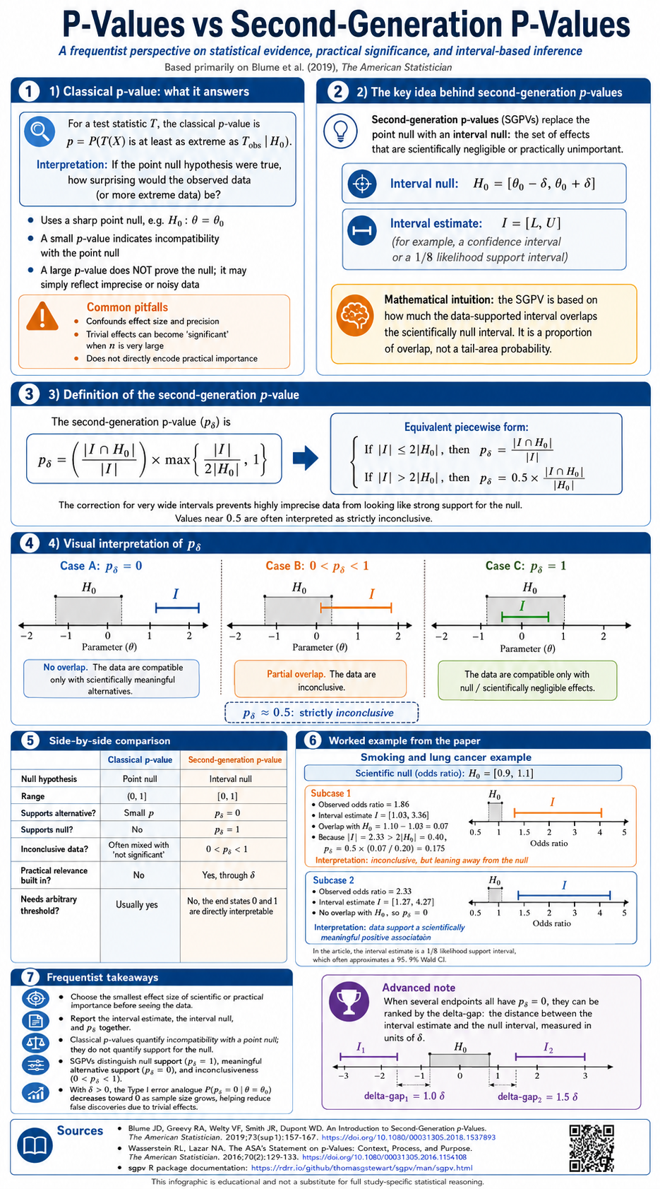
Infographic summary of the classical p-value workflow, second-generation p-value definition, visual interpretation, and worked examples. Click to open the full-size image.
Second-generation p-values are an attempt to make a frequentist summary answer a better scientific question. A traditional p-value asks how surprising a test statistic would be if a point null hypothesis were exactly true. The second-generation p-value asks how much of an interval estimate overlaps a scientifically meaningful null region.
That sounds like a small geometric change. It is not. It moves the analysis from "is the effect exactly zero?" to "does the data-supported effect region include values that are null or practically trivial?" It also creates an explicit third state: inconclusive evidence. For many real studies, that third state is the honest state.
The notation is usually , where indexes the interval null. If the interval null is , effects inside that band are treated as scientifically null or practically equivalent. If the effect scale is a ratio scale, the interval null is often defined symmetrically on the log scale, such as .
The Basic Definition
Let be an interval estimate for a parameter . This could be a confidence interval, likelihood support interval, compatibility interval, or credible interval; the SGPV machinery is geometric, though the operating characteristics depend on how the interval is constructed.
Let be the interval null. This is not merely a computational trick. It is the formal statement of what counts as no meaningful effect.
For finite intervals, the second-generation p-value is
The numerator is the length of overlap between the estimate interval and the interval null. The denominator prevents pathologies when one interval is much wider than the other. In the common finite-interval case implemented by sgpv::sgpvalue(), this leads to three interpretations:
p_delta = 0: the interval estimate does not overlap the interval null.0 < p_delta < 1: the interval estimate partly overlaps the interval null.p_delta = 1: the interval estimate is contained in the interval null.
When p_delta = 0, the sgpv package also reports a delta gap. This is the distance between the interval estimate and the interval null, standardized by half the null interval width. A large delta gap says the result is not merely outside the null region; it is separated from the null region by a practically interpretable margin.
library(sgpv)

sgpvalue(
  est.lo = 0.35,
  est.hi = 0.55,
  null.lo = -0.10,
  null.hi = 0.10
)
This is the simplest mental model: draw the interval null, draw the estimate interval, measure the overlap. The result is not a probability that the null is true. It is an interval compatibility index.

Original schematic recreated from the interval-overlap examples in public/sgpv/SGPV_ASA_Full_Day_Part1.Rmd and the local SGPV slide PDFs. The visual is redrawn rather than copied from a slide so the notation and styling match this article.
Why This Is Different From A Traditional p-Value
A traditional two-sided p-value is usually built from a statistic such as
and then reported as under the point null . In that construction, the reference distribution is generated under a point null, and the result is a tail area. A small p-value says that the observed statistic is unusual under that point null model.
That machinery is powerful, but it encourages several habits that statisticians have spent decades criticizing:
- It treats an exactly zero effect as the central inferential object even when exactly zero is scientifically implausible.
- It rewards precision enough to make tiny effects "significant."
- It does not distinguish "evidence for a null-sized effect" from "too little information to decide."
- It is often interpreted as though it were a posterior probability, which it is not.
SGPV keeps the frequentist interval-estimation frame but changes the inferential target. The interval null is chosen before looking at the data. The interval estimate carries uncertainty. Their overlap determines whether the evidence excludes, supports, or cannot distinguish scientifically null effects.
This makes SGPV especially natural for applied work where a smallest effect size of interest already exists: clinical non-inferiority margins, equivalence regions, minimum important differences, odds-ratio bands such as 0.9 to 1.11, fold-change thresholds in genomics, and policy thresholds where a tiny positive effect is not enough to act.
SGPVs do not convert frequentist intervals into posterior probabilities. A value of p_delta = 1 means the interval estimate lies inside the interval null; it does not mean the probability of the null is one. Likewise, p_delta = 0 means no overlap with the interval null; it is not the posterior probability that the effect is non-null.
Interpreting The Three Outcomes
The three SGPV outcomes are deliberately coarser than a traditional p-value. That coarseness is a feature when the goal is confirmatory scientific interpretation rather than continuous evidence ranking.
p_delta = 0
The interval estimate does not overlap the interval null. If the interval estimate was built with a frequentist confidence procedure, this behaves like a rule that rejects scientifically null effects only when the entire uncertainty interval lies outside the null region. The delta gap then quantifies how far away the interval is.
sgpvalue(
  est.lo = 0.35,
  est.hi = 0.55,
  null.lo = -0.10,
  null.hi = 0.10
)$delta.gap
0 < p_delta < 1
The interval estimate overlaps the interval null and also extends beyond it. This is the case that ordinary dichotomous testing handles poorly. SGPV labels it inconclusive. The data and design did not resolve whether the effect is null-sized or practically important.
sgpvalue(
  est.lo = 0.05,
  est.hi = 0.25,
  null.lo = -0.10,
  null.hi = 0.10
)$p.delta
p_delta = 1
The interval estimate is contained inside the interval null. This is evidence that the data-supported values are all null-sized or practically trivial, under the chosen interval construction and null region.
sgpvalue(
  est.lo = -0.04,
  est.hi = 0.04,
  null.lo = -0.10,
  null.hi = 0.10
)$p.delta
A Blood Pressure Toy Example
The local ASA workshop material uses a systolic blood pressure example with a point null of 145 mmHg and an interval null from 143 to 147 mmHg. The code appears in public/sgpv/SGPV_ASA_Full_Day_Part1.Rmd.
library(sgpv)

xbar <- c(141, 142, 143.5, 144, 146, 145, 145.5, 146) - 1
se <- c(0.5, 1, 0.5, 1, 2.25, 1.25, 0.25, 0.5)

delta.a <- 143
delta.b <- 147
h0 <- 145

lb <- xbar - 1.96 * se
ub <- xbar + 1.96 * se

sgp <- sgpvalue(
  est.lo = lb,
  est.hi = ub,
  null.lo = delta.a,
  null.hi = delta.b
)

raw_p <- 2 * pnorm(-abs((xbar - h0) / se))

data.frame(
  xbar = xbar,
  lo = lb,
  hi = ub,
  p_value = raw_p,
  p_delta = sgp$p.delta,
  delta_gap = sgp$delta.gap
)
The lesson is not that p-values are "wrong" and SGPVs are "right." The lesson is that the two columns answer different questions. The raw p-value asks about distance from 145 relative to standard error. The SGPV asks whether the interval estimate overlaps the scientifically null range 143 to 147.
Regression On Ratio Scales
Many regression outputs live on a ratio scale: odds ratios, risk ratios, hazard ratios. SGPV works best when the interval null is defined on a scale where symmetry makes scientific sense. For ratios, that usually means the log scale.
The workshop material includes a logistic-regression example with a null interval from 0.9 to 1.11 for odds ratios. On the log scale:
null.lo <- log(0.9)
null.hi <- log(1.11)

or_table <- data.frame(
  term = c(
    "treatment group",
    "tobacco",
    "microvascular obstruction",
    "dyslipidemia",
    "gender",
    "age",
    "hypertension"
  ),
  or = c(4.89, 4.59, 5.72, 2.32, 3.12, 1.02, 0.38),
  lo = c(1.18, 1.09, 0.86, 0.66, 0.36, 0.95, 0.09),
  hi = c(20.19, 19.28, 38.29, 8.98, 26.92, 1.11, 1.59),
  p_value = c(0.03, 0.04, 0.07, 0.22, 0.30, 0.56, 0.19)
)

sgp <- sgpvalue(
  est.lo = log(or_table$lo),
  est.hi = log(or_table$hi),
  null.lo = null.lo,
  null.hi = null.hi
)

cbind(or_table, p_delta = sgp$p.delta, delta_gap = sgp$delta.gap)
The age coefficient in the workshop example has an odds-ratio interval from 0.95 to 1.11, which sits inside the practical-null band 0.9 to 1.11. That is a different scientific statement than "the p-value is not small." A nonsignificant p-value can mean low precision; an SGPV of 1 means the whole interval estimate is inside the null region.
Plotting Intervals With plotsgpv()
The plotsgpv() function is designed for the visual diagnostic that SGPV naturally invites: show the interval estimates and overlay the interval null.
plotsgpv(
  est.lo = log(or_table$lo),
  est.hi = log(or_table$hi),
  null.lo = log(0.9),
  null.hi = log(1.11),
  set.order = order(or_table$p_value),
  null.pt = 0,
  outline.zone = TRUE,
  title.lab = "Logistic regression example",
  y.lab = "Log odds ratio",
  x.lab = "Classical p-value ranking",
  legend.on = TRUE
)
In the leukemia and simulated screening examples in the local workshop files, plotsgpv() is used to ask a highly practical question: among many intervals ranked by classical p-value, which ones actually exclude the interval null?
Original schematic recreated from the local leukemia and simulated screening examples in public/sgpv/SGPV_ASA_Full_Day_Part1.Rmd, especially the plotsgpv() and plotman() examples.
High-Dimensional Screening With plotman()
For many-testing workflows, the modified Manhattan-style plot is often more useful than a table. The workshop material simulates 10,000 screening features and compares the classical p-value axis with SGPV status.
set.seed(2026)
n_features <- 10000
pros.lo <- numeric(n_features)
pros.hi <- numeric(n_features)
pros.pvalue <- numeric(n_features)

for (i in seq_len(n_features)) {
  control <- runif(50, 0, 4)
  case <- runif(50, 0, 1.5)
  fit <- t.test(control, case)
  pros.pvalue[i] <- fit$p.value
  pros.lo[i] <- fit$conf.int[1]
  pros.hi[i] <- fit$conf.int[2]
}

plotman(
  est.lo = pros.lo,
  est.hi = pros.hi,
  null.lo = 0.5,
  null.hi = 1.3,
  set.order = NA,
  type = "delta-gap",
  title.lab = "Simulated screening example",
  y.lab = "Delta gap",
  x.lab = "Feature position",
  legend.on = TRUE
)

plotman(
  est.lo = pros.lo,
  est.hi = pros.hi,
  null.lo = 0.5,
  null.hi = 1.3,
  set.order = "sgpv",
  type = "comparison",
  p.values = -log10(pros.pvalue),
  ref.lines = -log10(0.05),
  title.lab = "Screening by SGPV status",
  y.lab = expression("-log"[10] * "(p-value)"),
  x.lab = "Second-generation p-value ranking",
  legend.on = TRUE
)
The inferential shift matters here. In a high-dimensional screen, a tiny p-value may still correspond to an effect interval that overlaps the null region if the null region is scientifically wide. Conversely, a slightly less extreme p-value may correspond to an interval that cleanly excludes null-sized effects.
Power, Type I Error, And Inconclusive Results
The sgpower() function computes operating characteristics when SGPV is the inferential metric.
sgpower(
  true = 0.5,
  null.lo = -0.1,
  null.hi = 0.1,
  std.err = 0.08,
  interval.type = "confidence",
  interval.level = 0.05
)
The key distinction is that SGPV operating characteristics have three buckets rather than two:
- probability of
p_delta = 0, often read as detecting a meaningful effect; - probability of
p_delta = 1, often read as confirming a null-sized effect; - probability of
0 < p_delta < 1, the inconclusive region.
That last probability is not a nuisance. It is the cost of being honest about precision and practical relevance. Designs with too little information should produce many inconclusive results; otherwise the procedure is pretending to know more than the data can support.
False Discovery Risk With fdrisk()
The fdrisk() function addresses a natural follow-up: after observing an SGPV of 0 or 1, how risky is that declaration under assumed null and alternative weighting distributions?
fdrisk(
  sgpval = 0,
  null.lo = log(1 / 1.1),
  null.hi = log(1.1),
  std.err = 0.8,
  null.weights = "Uniform",
  null.space = c(log(1 / 1.1), log(1.1)),
  alt.weights = "Uniform",
  alt.space = 2 + c(-1, 1) * qnorm(1 - 0.05 / 2) * 0.8,
  interval.type = "confidence",
  interval.level = 0.05
)
For sgpval = 0, the function returns a false discovery risk: the risk that a declared meaningful effect is actually null-sized under the specified weighting assumptions. For sgpval = 1, it returns a false confirmation risk: the risk that a declared null-sized effect is actually meaningfully non-null.
This is where the procedure becomes explicitly design-sensitive. SGPVs are not magic shields against poor design, poor measurement, or arbitrary null intervals. They make those decisions more visible.
Relationship To Equivalence And Non-Inferiority Testing
SGPV is closely related to equivalence logic, but it is not identical to a particular two-one-sided-tests workflow. Both approaches require a meaningful null or equivalence region. Both make scientific thresholds explicit. SGPV emphasizes the overlap of an interval estimate with the null region and returns a three-state result.
For example, the Part 2 workshop material compares TOST and SGPV in small-sample simulations:
library(TOSTER)
library(sgpv)

theta_p <- 0.5 * 0.75
theta_m <- -0.5 * 0.75

dat <- rnorm(6, 0, 1)
ci <- t.test(dat)$conf.int

sgpvalue(
  est.lo = ci[1],
  est.hi = ci[2],
  null.lo = theta_m,
  null.hi = theta_p
)
The practical lesson is that the interval-null definition should come first. The procedure is only as scientifically meaningful as the null region is defensible.
Choosing The Interval Null
This is the hardest part. It is also the part that makes SGPVs worth using.
A good interval null should be:
- chosen before looking at the study results;
- expressed on the correct scale, such as log odds ratio rather than odds ratio when symmetry matters;
- tied to a smallest effect size of scientific, clinical, policy, or operational interest;
- stable enough that readers can defend or dispute it directly;
- reported alongside sensitivity analyses when the threshold is uncertain.
Bad interval nulls are easy to spot. They are reverse-engineered after seeing the result, copied mechanically across unrelated domains, or defined on a scale where "equal distance" does not mean equal scientific change.
Applied Results Path
The following visual returns to the regression and screening examples. The first view orders intervals by classical p-value. The second orders by SGPV status. In a well-designed analysis, both views are worth inspecting: p-values are useful for tail-area ranking, but SGPVs ask whether the interval estimates clear the scientific null region.
A Practical Workflow
Here is the workflow I would use for a serious applied analysis:
- Define the estimand and effect scale.
- Define the interval null before inspecting estimates.
- Fit the model and report interval estimates.
- Compute SGPVs on the scientifically appropriate scale.
- Report
p_delta, delta gaps, and the original intervals. - Plot the intervals against the interval null.
- For high-dimensional screens, compare p-value ranking, adjusted p-values, SGPV status, and delta gaps.
- Run sensitivity analyses over plausible null interval widths.
- Use
sgpower()andfdrisk()during design or interpretation when operating characteristics matter.
SGPVs do not remove judgment from statistics. They put the judgment where it belongs: in the scientific definition of null-sized effects, the study design, and the interval estimate.
Sources
An Introduction to Second-Generation p-ValuesThe American Statistician introduction to second-generation p-values and their interpretation.
Second-generation p-values: Improved rigor, reproducibility, & transparency in statistical analysesBlume, D'Agostino McGowan, Dupont, and Greevy's PLOS ONE paper introducing the method and its motivation.
CRAN sgpv package documentation for sgpvalue()Reference documentation for computing SGPVs and delta gaps in R.
CRAN sgpv source for sgpvalue()Source code used to cross-check the finite-interval overlap formula implemented in the demo helper.
Local ASA workshop Part 1 RmdLocal support file used for the blood pressure, logistic regression, leukemia, plotsgpv(), and plotman() examples. Path in the repo: public/sgpv/SGPV_ASA_Full_Day_Part1.Rmd.
Local ASA workshop Part 2 RmdLocal support file used for sgpower(), fdrisk(), TOST comparison, and operating-characteristic examples.
Local SGPV introduction PDFThe local PDF supplied with this project. Its visual teaching structure informed the recreated schematics and live Motion workbench.
Motion for React documentationOfficial documentation for the installed Motion library used by the interactive components.
Motion Studio MCP install documentationOfficial Motion Studio MCP setup reference. The implementation uses the installed Motion library and cites the MCP docs because no Motion MCP server is exposed in this session.
Motion Studio AI context documentationOfficial notes on Motion Studio's AI context features, useful for reviewing the intended MCP-backed workflow.